Fatalities Model for Austria • bamlss

In this example we estimate a distributional regression model using data on fatalities in Austria. The data is taken from the Eurostat data base (https://ec.europa.eu/eurostat/) and includes weekly fatalities in Austria from the beginning of 2000 up to week~46 in 2020. The data is provided in the bamlss package and can be loaded with

data("fatalities", package = "bamlss")

The data set contains information on the number of fatalities (variable num) and the year and week of recording (variables year and week). The motivation for this analysis is to model a reference mortality, which allows one to describe the excess mortality caused by exceptional events such as pandemics (Leon et al. 2020) or natural catastrophes (Fouillet et al. 2008). Excess mortality refers to mortality in excess of what would be expected based on the non-crisis mortality rate in the population of interest. Here, we model the long-term seasonal trend of fatality numbers before the COVID-19 crisis and compare estimated quantiles with the cases in 2020, which will give insights into the excess mortality of the pandemic (Leon et al. 2020). Therefore, we subset the data set before 2020 for estimation and use the 2020 data for comparison

d19 <- subset(fatalities, year < 2020)
d20 <- subset(fatalities, year > 2019)

To find a well-calibrated model, the first step is to look for a suitable distribution for the data at hand. The gamlss.dist package (Stasinopoulos and Rigby 2019) provides a number of distributions which can also be used for estimation in bamlss. In this example, we consider 6 distributions with different number of parameters, from 2 to 4. In detail these are the normal distribution (family NO()), gamma and generalized gamma distribution (family GA() and GG()), Box-Cox t distribution (family BCT()), Box-Cox power exponential distribution (family BCPE()) and the Box-Cox Cole and Green distribution (family BCCG()). First, we only estimate the distributional parameters without covariates, to get a first idea which distribution fits well. We compare visually as well as by the deviance information criterion (DIC, the complete code is available here). Note that we do not use discrete distributions in this example because the number of fatalities is far away from zero in the thousands, i.e., a model for count data will most probable not improve the overall fit.

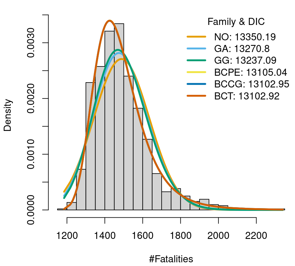
Fatalities data in Austria (2000–2019), histogram and fitted distributions.

One of the most flexible distributions of the gamlss.dist package, the four parameter Box-Cox t distribution, has a quite good fit and the lowest DIC (though only by a small difference). Hence, with some certainty one of the chosen distribution models will have a fairly good model fit in further analysis.

In the next step, we estimate Bayesian models that take into account the cyclical pattern over the year. In winter, there are usually quite a lot of influenza and other viral infections, which lead to a higher mortality rate. The models are estimated using the predictor \(\eta_k = f_{k} (\texttt{week})\) for each parameter of the distribution, where functions \(f_{k}(\texttt{week})\) are unspecified smooth functions, which are estimated using regression splines. We can use the following model formula for estimation

f <- list(
  num   ~ s(week, bs = "cc", k = 20),
  sigma ~ s(week, bs = "cc", k = 20),
  nu    ~ s(week, bs = "cc", k = 20),
  tau   ~ s(week, bs = "cc", k = 20)
)

again, function s() is the smooth term constructor from the mgcv package (Wood 2020) and bs = "cc" specifies a penalized cyclic cubic regression spline. Note that model formulae are provided as lists of formulae, i.e., each list entry represents one parameter of the response distribution. Since the maximum number of parameters of the selected distributions is 4, we supply 4 formulae. Internally, bamlss only processes the relevant formulae depending on the family. The gamlss.dist package has a naming convention for the distributional parameters, which is adopted in this example. However, the user can also drop the parameter names on the left hand side of the formulae (but not the response num). Moreover, note that all smooth terms, e.g., te(), ti(), are supported by bamlss. This way, it is also possible to incorporate user defined model terms, since the mgcv smooth term constructor functions are based on the generic smooth.construct() method, for which new classes can be added (see also the mgcv manual). For example, a full Bayesian semi-parametric distributional regression model using the BCPE() family of the gamlss.dist package can be estimated with

library("gamlss.dist")
set.seed(456)
b <- bamlss(f, data = d19, family = BCPE(mu.link = "log"),
  n.iter = 12000, burnin = 2000, thin = 10)

Note that we assign the log-link for parameter \(\mu\) to ensure positivity. In this example we use 12000 iterations for the MCMC sampler and withdraw the first 2000 samples and only save every \(10\)-th sample. We did the same estimation step analogously with the other distributions.

In addition to the DIC, there is also the Watanabe-Akaike information criterion (WAIC, Watanabe (2010)) to investigate the goodness of fit. In bamlss, the WAIC of the fitted model can be computed with

WAIC(b)

##     WAIC1    WAIC2       p1       p2
##  12184.73 12189.34 28.95351 31.25739

The function returns two values for the WAIC, depending on the type of the estimated number of parameters of the model (p1 uses expected differences of log densities, whereas p2 is computed using the variance in the log density, for details see Watanabe (2010)).

Another criterion for assessing model calibration is the continuous rank probability score (CRPS, Gneiting and Raftery (2007)). The R package scoringRules (Jordan, Krüger, and Lerch 2019) provides tools for model calibration checks using the CRPS. Since the number of candidate distributions can be quite large, it might happen that the CRPS for some distributions is not implemented. In this case, the user can resort to a numerical approximation as implemented in the function CRPS() in the bamlss package. Because the CRPS is a forecasting score, we computed the CRPS using 10-fold cross validation for each model. For example, the CRPS for the BCPE() model is computed with

set.seed(789)
folds <- rep(1:10, length.out = nrow(d19))
crps <- NULL
for(i in 1:10) {
  df <- subset(d19, folds != i)
  de <- subset(d19, folds == i)
  b3 <- bamlss(f, data = df, family = BCPE(mu.link = "log"),
    n.iter = 12000, burnin = 2000, thin = 10)
  crps <- c(crps, CRPS(b3, newdata = de, FUN = identity))
}
crps <- mean(crps)

The values of the DIC, WAIC and CRPS for the 6 models are

Family	DIC	WAIC	CRPS
`NO()`	12291.75	12294.20	51.89
`GA()`	12261.06	12262.40	51.72
`GG()`	12248.10	12249.31	51.52
`BCT()`	12215.85	12206.26	51.44
`BCCG()`	12190.41	12188.05	51.31
`BCPE()`	12188.30	12184.73	51.26

The table shows the DIC, WAIC and CRPS comparison of the 6 distributional cyclical week models. For the CRPS, 10-fold cross validation was used. Here, the four parameter BCPE() model has the lowest DIC, WAIC and CRPS, therefore, we examine this model in more detail in the rest of the analysis.

After the estimation algorithms are finished, the estimated effects, e.g., for the BCPE() model, can be visualized instantly using the plotting method.

plot(b, model = c("mu", "sigma", "nu", "tau"))

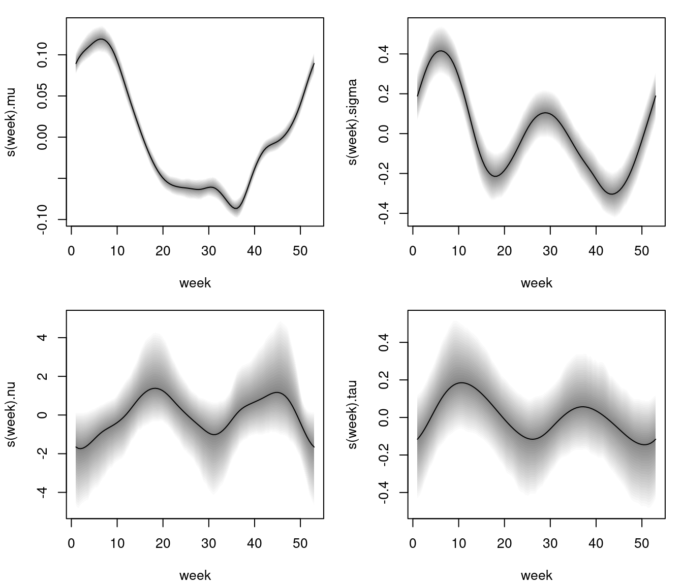
Estimated effects of week on parameter mu, sigma, nu and tau of the Box-Cox power exponential model. The grey shaded areas represent 95% credible intervals.

The estimated effects depict a clear nonlinear relationship for all parameters, however, 95% pointwise credible intervals for parameter nu and tau are larger such that the effects do not cross the horizontal zero line significantly, i.e., a simple intercept only specification for these parameters might be sufficient.

For judging how well the model fits to the data the user can inspect randomized quantile residuals (Dunn and Smyth 1996) using histograms or quantile-quantile (Q-Q) plots. Residuals can be extracted using function residuals() and has a plotting method. Alternatively, residuals can be investigated with

plot(b, which = "hist-resid")
plot(b, which = "qq-resid", c95 = TRUE)

Histogram and Q-Q plot including 95% credible intervals (dashed lines) of the resulting randomized quantile residuals of the distributional regression model.

By setting c95 = TRUE, the Q-Q plot includes 95% credible intervals. According the histogram and the Q-Q plot of the resulting randomized quantile residuals, the model seems to fit quite well.

In the next step, we compare quantiles of the intra-year long-term trend of the estimated distribution with the current situation in 2020. Therefore parameters for each week of the year are predicted

nd <- data.frame("week" = 1:53)
par <- predict(b, newdata = nd, type = "parameter")

and the estimated quantiles are computed with the quantile function of the family

nd$fit <- sapply(c(0.05, 0.5, 0.95),
  FUN = function(p) { family(b)$q(p, par) })

The estimated quantiles and the data used for modeling can now be plotted with

d19w <- reshape(d19, idvar = "week",
  timevar = "year", direction = "wide")
matplot(d19w$week, d19w[, -1],
  type = "b", lty = 1, pch = 16, col = gray(0.1, alpha = 0.1),
  xlab = "Week", ylab = "#Fatalities")
matplot(nd$week, nd$fit, type = "l", lty = c(2, 1, 2),
  col = 1, lwd = 3, add = TRUE)
lines(num ~ week, data = d20, col = 2, lwd = 2,
  type = "b", pch = 16, cex = 1.3)
grid()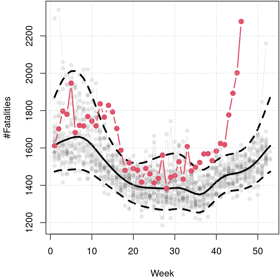

Predicted 5%, 50% and 95% quantiles of the cyclic seasonal week model, black lines, and number of fatalities in 2020 up to week 46, red points and line. Data before 2020 is shown in light gray in the background.

The resulting plot reveals the seasonal variation of fatalities. The median reveals a clear annual cycle with a higher number of fatalities in winter. The skewness of the distribution is also very dominant in winter. However, also in the summer months there is a visible increase in the upper quantile, which is probably due to particular heat waves leading to greater cardiovascular stress (Fouillet et al. 2008). The mortality rate from beginning of 2020 to week 46 is plotted in red and clearly indicates that this is much higher than the long-term median in the spring and from about week 40 onward, and also well above the estimated 95% quantile, respectively.

Dunn, Peter K., and Gordon K. Smyth. 1996. “Randomized Quantile Residuals.” Journal of Computational and Graphical Statistics 5 (3): 236–44. https://doi.org/10.2307/1390802.

Fouillet, A, G Rey, V Wagner, K Laaidi, P Empereur-Bissonnet, A Le Tertre, P Frayssinet, et al. 2008. “Has the Impact of Heat Waves on Mortality Changed in France Since the European Heat Wave of Summer 2003? A Study of the 2006 Heat Wave.” International Journal of Epidemiology 37 (2): 309–17. https://doi.org/10.1093/ije/dym253.

Gneiting, Tilmann, and Adrian E. Raftery. 2007. “Strictly Proper Scoring Rules, Prediction, and Estimation.” Journal of the American Statistical Association 102 (477): 359–78. https://doi.org/10.1198/016214506000001437.

Jordan, Alexander, Fabian Krüger, and Sebastian Lerch. 2019. “Evaluating Probabilistic Forecasts with scoringRules.” Journal of Statistical Software 90 (12): 1–37. https://doi.org/10.18637/jss.v090.i12.

Leon, David A, Vladimir M Shkolnikov, Liam Smeeth, Per Magnus, Markéta Pechholdová, and Christopher I Jarvis. 2020. “COVID-19: A Need for Real-Time Monitoring of Weekly Excess Deaths.” The Lancet 395 (10234): e81. https://doi.org/https://doi.org/10.1016/S0140-6736(20)30933-8.

Stasinopoulos, Mikis, and Robert Rigby. 2019. Gamlss.dist: Distributions for Generalized Additive Models for Location Scale and Shape. https://CRAN.R-project.org/package=gamlss.dist.

Umlauf, Nikolaus, Nadja Klein, Achim Zeileis, and Thorsten Simon. 2024. bamlss: Bayesian Additive Models for Location Scale and Shape (and Beyond). https://CRAN.R-project.org/package=bamlss.

Watanabe, Sumio. 2010. “Asymptotic Equivalence of Bayes Cross Validation and Widely Applicable Information Criterion in Singular Learning Theory.” The Journal of Machine Learning Research 11: 3571–94.

Wood, S. N. 2020. mgcv: GAMs with Gcv/Aic/Reml Smoothness Estimation and Gamms by Pql. https://CRAN.R-project.org/package=mgcv.