Plot Maps
plotmap.RdThe function takes a list polygons and draws the corresponding map. Different
colors for each polygon can be used.
plotmap(map, x = NA, id = NULL, select = NULL,
  legend = TRUE, names = FALSE, values = FALSE, ...)
Arguments
- map
The map to be plotted, usually an object that inherits from
SpatialPolygons, but may also be a list of polygons, i.e., each list entry is a matrix with x- and y-coordinates.- x
A vector, data.frame or matrix. In the latter case
xshould have two columns, one column that is the region identifier and one that contains the values to be plotted. In casexis a data.frame, the function searches for"character"or"factor"columns for the region identifier. Ifxis a matrix, the second column ofxis supposed to be the region identifier. Ifx = NAandmapis an object of class"SpatialPolygonsDataFrame"only the polygons will be plotted without using the data.- id
If argument
xis a vector, argumentidshould contain the region identifier vector.- select
Select the column of the data in
xwhich should be used for plotting, may be an integer or character with the corresponding column name.- legend
Should a color legend be added to the plot, see also function
colorlegend.- names
If set to
TRUEthe name for each polygon will also be plotted at the centroids of the corresponding polygons.- values
If set to
TRUEthe corresponding values for each polygon will also be plotted at the centroids of the polygons.- ...
Arguments to be passed to
colorlegendand others, e.g. change theborderof the polygons anddensity(mdensityfor missing regions inid), seepolygon.
Examples
## Example from mgcv ?mrf.
## Load Columbus Ohio crime data (see ?columbus for details and credits).
data("columb", package = "mgcv")
data("columb.polys", package = "mgcv")
## Plot the map.
plotmap(columb.polys)
 ## Plot aggregated data.
a <- with(columb, aggregate(crime,
by = list("district" = district), FUN = mean))
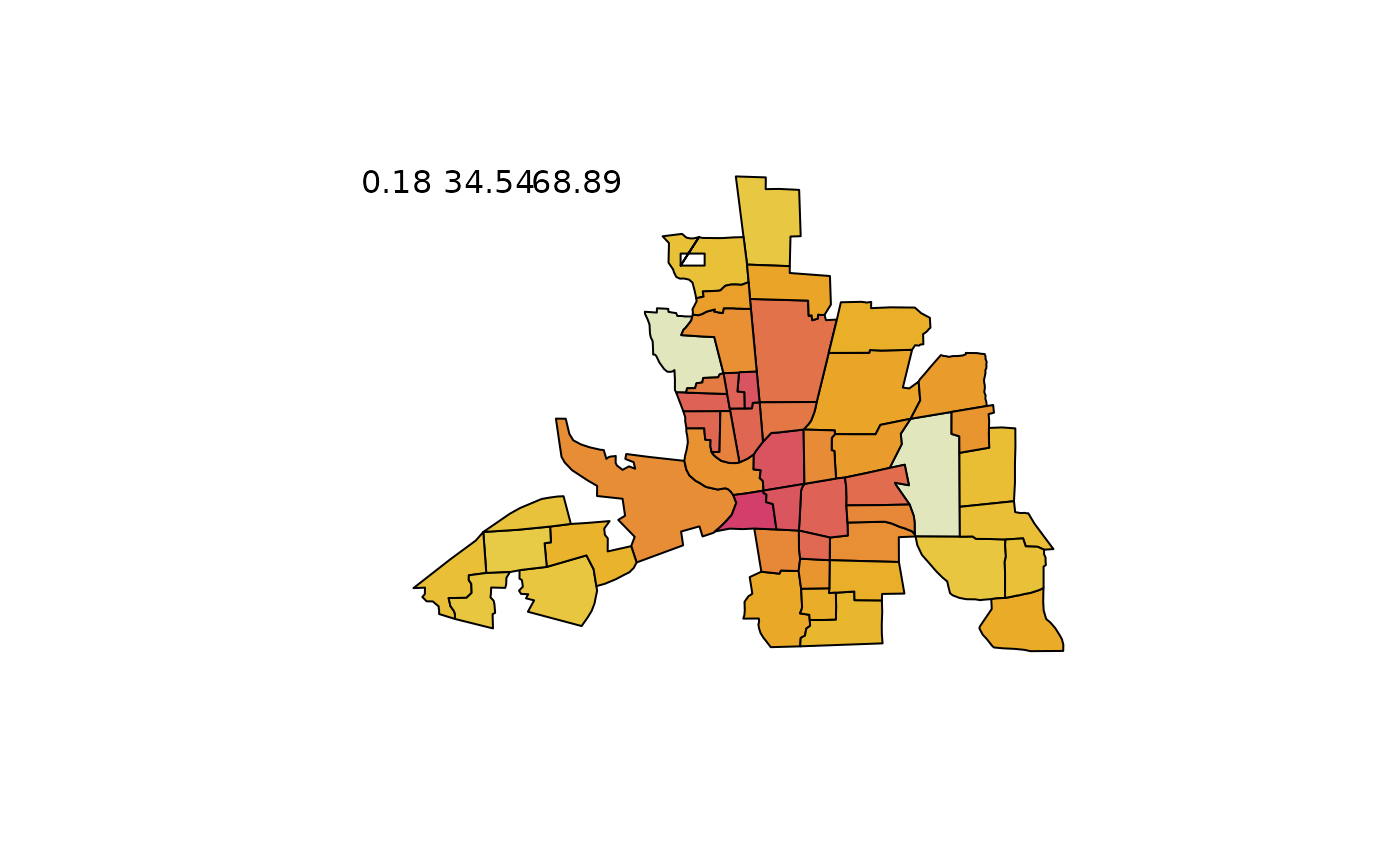
plotmap(columb.polys, x = a$x, id = a$district)
 plotmap(columb.polys, x = a$x, id = a$district,
pos = "topleft")
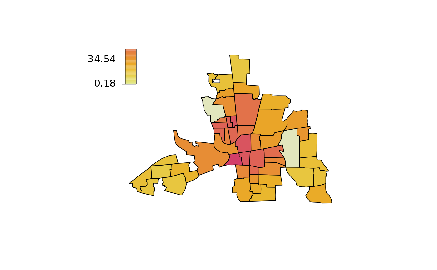
plotmap(columb.polys, x = a$x, id = a$district,
pos = "topleft", side.legend = 2)
plotmap(columb.polys, x = a$x, id = a$district,
pos = "topleft")
plotmap(columb.polys, x = a$x, id = a$district,
pos = "topleft", side.legend = 2)
 plotmap(columb.polys, x = a$x, id = a$district,
pos = "topleft", side.legend = 2, side.ticks = 2)
 plotmap(columb.polys, x = a$x, id = a$district,
pos = "topleft", side.legend = 2, side.ticks = 2,
col = heat_hcl, swap = TRUE)
plotmap(columb.polys, x = a$x, id = a$district,
pos = "topleft", side.legend = 2, side.ticks = 2,
col = heat_hcl, swap = TRUE, range = c(10, 50))
plotmap(columb.polys, x = a$x, id = a$district,
pos = "topleft", side.legend = 2, side.ticks = 2,
col = heat_hcl, swap = TRUE)
plotmap(columb.polys, x = a$x, id = a$district,
pos = "topleft", side.legend = 2, side.ticks = 2,
col = heat_hcl, swap = TRUE, range = c(10, 50))
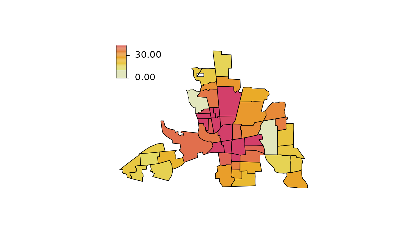
 plotmap(columb.polys, x = a$x, id = a$district,
pos = "topleft", side.legend = 2, side.ticks = 2,
col = heat_hcl(5), swap = TRUE, range = c(10, 50),
lrange = c(0, 60))
