Plot Slices of Bivariate Functions
sliceplot.RdThis function plots slices from user defined values of bivariate surfaces.
sliceplot(x, y = NULL, z = NULL, view = 1, c.select = NULL,
  values = NULL, probs = c(0.1, 0.5, 0.9), grid = 100,
  legend = TRUE, pos = "topright", digits = 2, data = NULL,
  rawdata = FALSE, type = "mba", linear = FALSE,
  extrap = FALSE, k = 40, rug = TRUE, rug.col = NULL,
  jitter = TRUE, ...)
Arguments
- x
A matrix or data frame, containing the covariates for which the effect should be plotted in the first and second column and at least a third column containing the effect. Another possibility is to specify the plot via a
formula, e.g., for simple plotting of bivariate surfacesz ~ x + y, see the examples.- y
If
xis a vector the argumentyandzmust also be supplied as vectors.- z
If
xis a vector the argumentyandzmust also be supplied as vectors,zdefines the surface given by \(z = f(x, y)\).- view
Which variable should be used for the x-axis of the plot, the other variable will be used to compute the slices. May also be a
characterwith the name of the corresponding variable.- c.select
Integer, selects the column that is used in the resulting matrix to be used as the
zargument.- values
The values of the
xoryvariable that should be used for computing the slices, if set toNULL, slices will be constructed according to the quantiles, see also argumentprobs.- probs
Numeric vector of probabilities with values in [0,1] to be used within function
quantileto compute thevaluesfor plotting the slices.- grid
The grid size of the surface where the slices are generated from.
- legend
If set to
TRUE, a legend with thevaluesthat where used for slicing will be added.- pos
The position of the legend, see also function
legend.- digits
The decimal place the legend values should be rounded.
- data
If
xis aformula, adata.frameorlist. By default the variables are taken fromenvironment(x): typically the environment from whichplot3dis called.- rawdata
If set to
TRUE, the data will not be interpolated, only raw data will be used. This is useful when displaying data on a regular grid.- type
Character, which type of interpolation method should be used. The default is
type = "akima", see functioninterp. The two other options aretype = "mba", which calls functionmba.surfof package MBA, ortype = "mgcv", which uses a spatial smoother withing package mgcv for interpolation. The last option is definitely the slowest, since a full regression model needs to be estimated.- linear
Logical, should linear interpolation be used withing function
interp?- extrap
Logical, should interpolations be computed outside the observation area (i.e., extrapolated)?
- k
Integer, the number of basis functions to be used to compute the interpolated surface when
type = "mgcv".- rug
Add a
rugto the plot.- jitter
- rug.col
Specify the color of the rug representation.
- ...
Details
Similar to function plot3d, this function first applies bivariate interpolation
on a regular grid, afterwards the slices are computed from the resulting surface.
Note
Function sliceplot can use the akima package to construct smooth interpolated
surfaces, therefore, package akima needs to be installed. The akima package has an ACM
license that restricts applications to non-commercial usage, see
https://www.acm.org/publications/policies/software-copyright-notice
Function sliceplot prints a note referring to the ACM license. This note can be suppressed by
setting
options("use.akima" = TRUE)
Examples
## Generate some data.
set.seed(111)
n <- 500
## Regressors.
d <- data.frame(z = runif(n, -3, 3), w = runif(n, 0, 6))
## Response.
d$y <- with(d, 1.5 + cos(z) * sin(w) + rnorm(n, sd = 0.6))
if (FALSE) ## Estimate model.
b <- bamlss(y ~ te(z, w), data = d)
summary(b)
#> Error in eval(expr, envir, enclos): object 'b' not found
## Plot estimated effect.
plot(b, term = "te(z,w)", sliceplot = TRUE)
#> Error in h(simpleError(msg, call)): error in evaluating the argument 'x' in selecting a method for function 'plot': object 'b' not found
plot(b, term = "te(z,w)", sliceplot = TRUE, view = 2)
#> Error in h(simpleError(msg, call)): error in evaluating the argument 'x' in selecting a method for function 'plot': object 'b' not found
plot(b, term = "te(z,w)", sliceplot = TRUE, view = "w")
#> Error in h(simpleError(msg, call)): error in evaluating the argument 'x' in selecting a method for function 'plot': object 'b' not found
plot(b, term = "te(z,w)", sliceplot = TRUE, probs = seq(0, 1, length = 10))
#> Error in h(simpleError(msg, call)): error in evaluating the argument 'x' in selecting a method for function 'plot': object 'b' not found
## Variations.
d$f1 <- with(d, sin(z) * cos(w))
sliceplot(cbind(z = d$z, w = d$w, f1 = d$f1))
 ## Same with formula.
sliceplot(sin(z) * cos(w) ~ z + w, ylab = "f(z)", data = d)
## Same with formula.
sliceplot(sin(z) * cos(w) ~ z + w, ylab = "f(z)", data = d)
 ## Compare with plot3d().
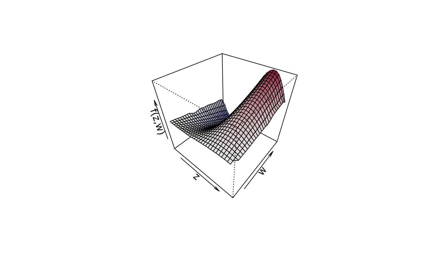
plot3d(sin(z) * 1.5 * w ~ z + w, zlab = "f(z,w)", data = d)
## Compare with plot3d().
plot3d(sin(z) * 1.5 * w ~ z + w, zlab = "f(z,w)", data = d)
 sliceplot(sin(z) * 1.5 * w ~ z + w, ylab = "f(z)", data = d)
 sliceplot(sin(z) * 1.5 * w ~ z + w, view = 2, ylab = "f(z)", data = d)
